Tutorial
Basic Usage
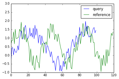
Firstly, let’s generate toy data for this tutorial.
import numpy as np
import matplotlib.pyplot as plt

np.random.seed(1234)
# generate toy data
x = np.sin(2 * np.pi * 3.1 * np.linspace(0, 1, 101))
x += np.random.rand(x.size)
y = np.sin(2 * np.pi * 3 * np.linspace(0, 1, 120))
y += np.random.rand(y.size)

plt.plot(x, label="query")
plt.plot(y, label="reference")
plt.legend()
plt.ylim(-1, 3)
Then run dtw() method which returns DtwResult object.
from dtwalign import dtw
res = dtw(x, y)
Note
The first run takes a few seconds for jit compilation.
DTW distance
DTW distance can be refered via DtwResult object.
print("dtw distance: {}".format(res.distance))
# dtw distance: 30.048812654583166
print("dtw normalized distance: {}".format(res.normalized_distance))
# dtw normalized distance: 0.13596747807503695
Note
If you want to calculate only dtw distance (i.e. no need to gain alignment path), give ‘distance_only’ argument as True when runs dtw method (it makes faster).
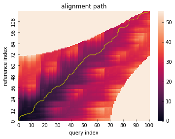
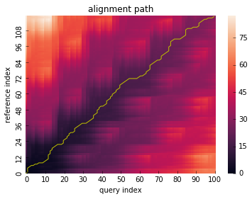
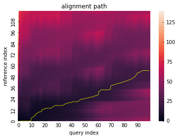
Alignment path
DtwResult object offers a method which visualize alignment path with cumsum cost matrix.
res.plot_path()
Alignment path array is also provided:
x_path = res.path[:, 0]
y_path = res.path[:, 1]
Warp one to the other
get_warping_path() method provides an alignment path of X with fixed Y and vice versa.
# warp x to y
x_warping_path = res.get_warping_path(target="query")
plt.plot(x[x_warping_path], label="aligned query to reference")
plt.plot(y, label="reference")
plt.legend()
plt.ylim(-1, 3)
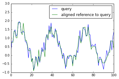
# warp y to x
y_warping_path = res.get_warping_path(target="reference")
plt.plot(x, label="query")
plt.plot(y[y_warping_path], label="aligned reference to query")
plt.legend()
plt.ylim(-1, 3)
Advanced Usage
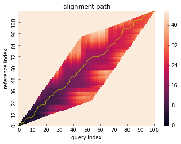
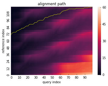
Global constraint
dtw() method can take window_type parameter to constrain
the warping path globally which is also known as ‘windowing’.
# run DTW with Itakura constraint
res = dtw(x, y, window_type="itakura")
res.plot_path()
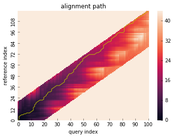
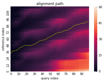
# run DTW with Sakoechiba constraint
res = dtw(x, y, window_type="sakoechiba", window_size=20)
# visualize alignment path with cumsum cost matrix
res.plot_path()
Local constraint
dtwalign package also supports local constrained optimization
which is also known as ‘step pattern’.
Following step patterns are supported:
- symmetric1
- symmetric2
- symmetricP05
- symmetricP0
- symmetricP1
- symmetricP2
- Asymmetric
- AsymmetricP0
- AsymmetricP05
- AsymmetricP1
- AsymmetricP2
- TypeIa
- TypeIb
- TypeIc
- TypeId
- TypeIas
- TypeIbs
- TypeIcs
- TypeIds
- TypeIIa
- TypeIIb
- TypeIIc
- TypeIId
- TypeIIIc
- TypeIVc
- Mori2006
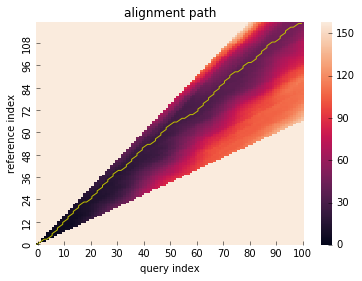
# run DTW with symmetricP2 pattern
res = dtw(x, y, step_pattern="symmetricP2")
res.plot_path()
Partial alignment
dtw() method also be able to perform partial matching algorithm
by setting open_begin and open_end.
Before see example code, let’s make toy data via following:
x_partial = np.sin(2 * np.pi * 3 * np.linspace(0.3, 0.8, 100))
x_partial += np.random.rand(x_partial.size)
y_partial = np.sin(2 * np.pi * 3.1 * np.linspace(0, 1, 120))
y_partial += np.random.rand(y_partial.size)

plt.plot(x_partial, label="query")
plt.plot(y_partial, label="reference")
plt.legend()
plt.ylim(-1, 3)
Open-end alignment can be performed by letting open_end be True.
res = dtw(x_partial, y_partial, open_end=True)
res.plot_path()
As above, let open_begin be True to run open-begin alignment.
Note
Open-begin requires “N” normalizable pattern. If you want to know more detail, see references.
res = dtw(x_partial, y_partial, step_pattern="asymmetric", open_begin=True)
res.plot_path()
res = dtw(x_partial, y_partial, step_pattern="asymmetric", open_begin=True, open_end=True)
res.plot_path()
Use other metric
You can use other pair-wise distance metric (default is euclidean).
Metrics in scipy.spatial.distance.cdist are supported:
res = dtw(x, y, dist="minkowski")
Arbitrary function which returns distance value between x and y is also available.
res = dtw(x, y, dist=lambda x, y: np.abs(x - y))
Use pre-computed distance matrix
You can also calculate DTW with given pre-computed distance matrix like:
# calculate pair-wise distance matrix in advance
from scipy.spatial.distance import cdist
X = cdist(x[:, np.newaxis], y[:, np.newaxis], metric="euclidean")

# use `dtw_from_distance_matrix` method for computation.
from dtwalign import dtw_from_distance_matrix
res = dtw_from_distance_matrix(X, window_type="itakura", step_pattern="typeIVc")
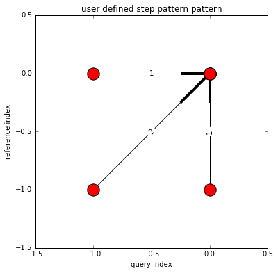
Use user-defined constraints
Local constraint (step pattern)
# define local constraint (step pattern)
from dtwalign.step_pattern import UserStepPattern
pattern_info = [
                    dict(
                        indices=[(-1,0),(0,0)],
                        weights=[1]
                    ),
                    dict(
                        indices=[(-1,-1),(0,0)],
                        weights=[2]
                    ),
                    dict(
                        indices=[(0,-1),(0,0)],
                        weights=[1]
                    )
                ]
user_step_pattern = UserStepPattern(pattern_info=pattern_info,normalize_guide="N+M")

# plot
user_step_pattern.plot()
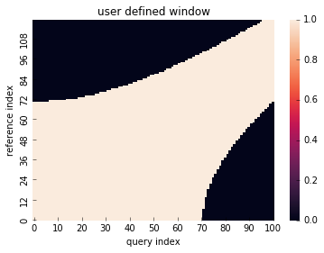
Global constraint (windowing)
# define global constraint (windowing)
from dtwalign.window import UserWindow
user_window = UserWindow(X.shape[0], X.shape[1], win_func=lambda i, j: np.abs(i ** 2 - j ** 2) < 5000)

# plot
user_window.plot()
To compute DTW with user-specified constraints, use dtw_low method like:
# import lower dtw interface
from dtwalign import dtw_low
res = dtw_low(X,window=user_window,pattern=user_step_pattern)
res.plot_path()